Master Activity 1

Complete the following Master Activity and submit your completed project.

Google Sheets

You will need to be logged into Google account to complete this assignment. Since Google Sheets is web based, it changes frequently. The steps outlined here may be slightly different from what you see on your screen. If you do not already have a Google account, you will need to create one. Go to http://google.com and in the upper right corner, click Sign In. On the Sign in screen, click Create Account. On the Create your Google Account page, complete the form, read and agree to the Terms of Service and Privacy Policy, and then click Next step. On the Welcome screen, click Get Started.

1. From the desktop, open your browser, navigate to http://google.com, and then sign in to your Google account. In the upper right corner of your screen, click Google apps, and then click Drive. If you are already logged into Google click Apps, then Sheets.
2. Click Blank to open a new untitled sheet.
3. In the left pane, click New, and then click Google Sheets to open a new tab in your browser and to start an Untitled sheet. At the top of the window, click Untitled sheet and then, using your own name as the file name, type Lastname_Firstname_ExcelMaster1 and then press Enter to change the file name.
4. To the right of the file name, point to the small file folder to display the ScreenTip Move to. Click the file folder and notice that your file is saved in the OFTEC 108 folder.
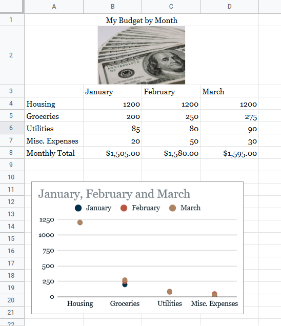
5. In cell A1, type My Budget By Month and press Enter.
6. In cell A2 Type For the First Quarter and press Enter.
7. In Cell A4, Type each of the following, pressing Enter after each:
   • Housing
   • Groceries
   • Utilities
   • Misc Expenses
   • Monthly Total
8. In cell B3, type January and press Enter.
9. Select cell B3 and use the fill handle to drag to cell E3. Notice how the names of the months automatically generate. The fill handle enables auto fill, which generates and extends a series of values into adjacent cells based on the value of other cells.
10. Select cell E3 and press the Delete key.
11. Select the range B4:D7 and enter the following text, pressing the tab key after each number.

12. With cell B8 active go to the Insert tab, Function and choose SUM. Click in cell B4 and drag down to cell B7 and press Enter. With cell B8 selected, notice the formula bar shows =SUM(B4:B7), and the formula result also displays here. Press Enter if necessary.
13. With cell B8 selected, use the fill handle to fill the formula to cells C8 and D8.
14. Select the range A3:D7, be sure not to include the Totals.
15. On the Insert Tab, choose Chart, and notice how a clustered column chart is added.
16. Resize and move the chart so that the upper left hand corner fits in cell A10 and the lower right hand corner fits in cell E21.
17. Select the chart, and choose the Ellipsis, which is the three small dots in the upper right hand corner of the chart. This will open the Chart Editor.
18. In the chart editor, under Setup, select the arrow next to Chart Type to display all chart types. If you do not have access to Setup, continue on to step 20.
19. Select any chart other than the Clustered Column Chart. Close the Chart Editor.
20. On the Format tab, select Theme and choose the Streamline theme. Close Themes.
21. Select the range A1:D1 and merge the cells, and then align center. This is on the format tab.
22. Select the range A2:D2 and merge the cells, and then align center.
23. Select cell A2. On the Insert tab, select Image, Image in Cell. In the Insert Image dialog box, scroll to the right until you see Google Image Search. Select this, and in the Search For box type Money then press Enter. Select any picture and then click insert.
24. Resize cell A2 by dragging the line between the 2 and 3 down. Center align the image in the cell.
25. Select the range B8:D8 and format the text as Currency. This is under Format.
26. Click Tools, Spelling, Spell Check. Verify Spelling and Grammar is correct.
27. Take a moment to preview your document, and make any adjustments as necessary. Ensure your document will be saved automatically. Submit as instructed by your instructor.