Challenge It

In this challenge activity, you will complete a project that incorporates many of the key skills learned in the Excel Unit. For this project, you are an IT manager responsible for managing the technology inventory for your college.

1. Open the Excel spreadsheet Starter_Excel_Challenge. Save the file to your flash drive or other safe location as designated by your instructor and name the file Lastname_Firstname_Excel_Challenge.
2. Merge and center the text in cell A1 across the range A1:G1 and apply the cell style Heading 2.
3. Merge and center the text in cell A2 across the range A2:G2 and apply the cell style Heading 4.
4. Apply the Title cell style to the range A11:F11.
5. Autofit all cell contents, both column widths and row heights, if necessary.
6. In cell B4, construct a function to SUM the total quantity in stock.
7. In cell B5, construct a function that will find the AVERAGE price (or value) of all of the items. Format as currency with two decimal places.
8. In cell B6, construct a function that will find the MEDIAN price (or value) of all items. Format as currency with two decimal places.
9. In cell B7, construct a function that will find the lowest of MIN price (or value) for all items. Format as currency with two decimal places.
10. In cell B8, construct a function that will find the highest of MAX price (or value) for all items. Format as currency with two decimal places.
11. Format the Values in column C as currency with two decimal places.
12. Select the range A4:B9, and move it to F4:G9.
13. Insert a new column after column B and label it Item Type.
14. Insert another new column before Column C and label it Item #. Your new Column C should be Item # and Column D should be Item Type.
15. In cell C12, use Flash fill to list the Item # from column B in column C.
16. In cell D12, use Flash Fill to list the Item Type from column B in column D.
17. Select column B and delete it. If necessary, move cells G4:H9 back over to cells F4:G9.
18. In cell G9, construct a function that will count the number of Laptop Categories.
19. Select the range F4:G9 and move to the range back to A4:B9 and apply the 20% Accent 1 cell style.
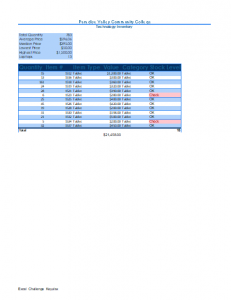
20. In cell F12, construct a function that will determine if the stock level is ok, or needs to be checked. The threshold for the stock level is 7. If the quantity is less than 7, then it needs to be checked. Use “Check” and “OK” as the true and false values. Use the fill handle to fill the function to cell F47.
21. Use conditional formatting, highlight cells rule, text that contains “Check”. Format the text with Light Red Fill with Dark Red Text.
22. Run Spelling and Grammar check.
23. Rename Sheet1 to Inventory.
24. Add a new sheet and name it Summary.
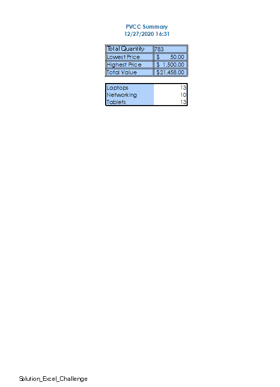
25. On the Summary Sheet, in cell A1 type PVCC Summary.
26. In cell A2, construct a formula that will display the current day and time.
27. Merge and center the text in cell A1 across the range A1:B1 and apply the cell style Heading 4.
28. Merge and center the text in cell A2 across the range A2:B2 and apply the cell style Heading 4.
29. In cell A4, type Total Quantity.
30. In cell B4 on the Summary Sheet, enter a formula that will reference the Total Quantity in cell B4 on the Inventory Sheet.
31. In cell A5 on the Summary Sheet, type Lowest Price.
32. In cell B5 on the Summary Sheet, enter a formula that will reference the Lowest Priced item in cell B7 on the Inventory Sheet.
33. In cell A6 on the Summary Sheet, type Highest Price.
34. In cell B6 on the Summary Sheet, enter a formula that will reference the Highest Priced item in cell B8 on the Inventory Sheet.
35. In cell B7 on the Summary Sheet, construct a formula that will calculate the Total value by summing the Value on the Inventory sheet. Type the label Total Value in cell A7.
36. Select the range A4:B7 on the Summary Sheet, and left align. If necessary, autofit the cell contents so that all of the values are visible. Apply the 20% Accent 1 cell style to the range.
37. On the Inventory Tab, select the range A11:F47 and format as a table with headers.
38. Apply a filter to the category field so that only Laptops display. Add a total row to the table. Below the table in column D, add the sum of the D12 to D47 in cell D49. 
39. On the Summary sheet in cell A9 type Laptops. In cell B9, type the total number of laptops that displays on the Inventory Sheet.
40. On the Inventory Sheet, apply a filter to the category field so that only Networking displays.
41. On the Summary sheet in cell A10 type Networking. In cell B10, type the total number of networking items that display on the Inventory Sheet.
42. On the Inventory Sheet, apply a filter to the category field so that only Tablets display.
43. On the Summary sheet in cell A11, type Tablets. In cell B11 type the total number of Tablets that displays on the Inventory Sheet.
44. On the Summary sheet, place a thick outside border around the range A9:B11.
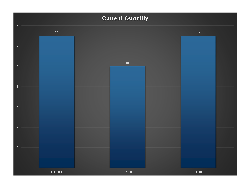
45. On the Summary sheet, select the range A9:B11 and insert the Clustered Column recommended chart.
46. Move the Chart to its own sheet named Chart.
47. Change the Chart Title to Current Quantity.
48. Apply Chart Style 9 and change colors to the first one under Monochromatic.
49. Apply Data Labels in the Center position to the Chart.
50. Add a new sheet to the workbook, and name it Trend.
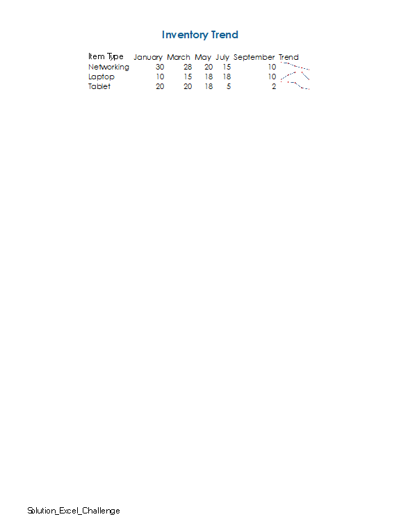
51. In cell A1 type Inventory Trend. Merge and Center it across the range A1:G1 and apply the Heading 1 cell style.
52. In cell A3, type Item Type.
53. In cell B3, type January and press tab. In cell C3 type March and press tab.
54. Select the range B3:B4, and use the fill handle to fill the range to cell F3.
55. In cell A4 type Networking, in cell A5 type Laptop, and in cell A6 type Tablet.
56. On the Trend sheet, continue to enter the following data:

57. Select the range A3:F6 and apply the slice theme and autofit all cell content.
58. In cell G3, type Trend.
59. In cell G4, add a sparkline that shows the trend for January-September. Apply markers, and use the fill handle to copy the sparkline to the cells G5 and G6.
60. Reorder the sheets so that they are in this order: Summary, Trend, Chart, Inventory.
61. Group all 4 sheets and launch the Page Setup Dialog Box.
62. Apply the following on the Page Setup Dialog Box:
    • Fit to 1 page
    • Center horizontally on page
    • Insert the File Name in the Footer on the left side
63. Ungroup the sheets and apply the following advanced properties:
    • Title: Excel Challenge
    • Subject: OFTEC 108 and section #
    • Author: Your first and last name
    • Keywords: Charts, Functions, Sparklines
64. View the print preview, and make any modifications based on the images below.
65. Run a spelling and grammar check, and submit your file based on your instructor’s instructions.