Excel Practice 1

Since Microsoft Excel is widely used in industry, and we are using Microsoft Windows, we will focus on Excel going forward. There are many similarities across spreadsheet software, so the skills we are learning can be translated to other software and apps. The following ‘Practice It’ assignments are designed to be completed using Microsoft Excel in Office 365 on a PC with Windows 10 or higher.

We will use Excel to perform complex calculations, analyze data so that we can make intelligent decisions, and create visually interesting charts and graphs that help us understand the data. Since Excel is used for Data Analysis, it is best to use a keyboard and mouse or touchpad rather than the touchscreen.

In Excel, data is stored in a cell. Cell content is anything that is stored in the cell and can be either a constant value or a formula. The most commonly used values are text values and number values. Values can also be a date or time. A text value is also referred to as a label.

Here is a video demonstrating the skills in this practice. Please note it does not exactly match the instructions: 

Complete the following Practice Activity and submit your completed project.

For our first assignment in Excel, we will create a spreadsheet with monthly expenses. This spreadsheet will provide us with an overall picture of our financial health by helping us understand where we are spending our hard-earned money. We will start with a new blank Excel Spreadsheet.

1. Start Excel. Click Blank Workbook.
2. Select File, Save As, Browse, and then navigate to your Excel folder on your flash drive or other location where you save your files. Name the workbook as Yourlastname_Yourfirstname_Excel_Practice_1.
3. Take a moment to locate the following components of the Excel workbook window. Notice how Columns are lettered and Rows are numbered. The intersection of a row and column is a cell. The active cell in the image is A1.
4. Notice the vertical and horizontal scroll bars. Use the arrows to practice scrolling on the page.
5. In cell A1, type My Budget By Month and press Enter.
6. In cell A2 Type For the First Quarter and press Enter.
7. In the Name Box, change A3 to A4 and then press Enter. Notice how the active cell changed to A4.
8. Starting in cell A4, Type each of the following (excluding the circle bullets), pressing Enter after each:
   • Housing
   • Groceries
   • Utilities
   • Misc Expenses
   • Monthly Total
9. In cell B3, type January and press Enter.
10. Select cell B3 and use the fill handle to drag to cell D3. Notice how the names of the months automatically generate. The fill handle enables auto fill, which generates and extends a series of values into adjacent cells based on the value of other cells.

11. Adjust the column width for column A to 136 pixels by dragging the right boundary (between columns A and B) to the right.
12. Select the range B3:D3 and center the text.

13. In cell B4, type 1200 and enter the remaining numbers as shown:

14. In cell B8, type =b4 + b5 + b6 + b7 and press Tab.
15. In cell C8, type =c4 + c5 + c6 + c7 and press Tab.

16. A quicker way to enter in a formula is with a function. We will use the SUM function next. In cell D8, click AutoSum on the Home Tab, Editing Group and press Enter.
17. In cell E3, type Total and then press Enter.
18. Click in cell E4, Press Alt + =. This is a keyboard shortcut that enters the Sum function. If the keyboard shortcut does not work (this is common due to variations in keyboards), use the AutoSum technique from step 16.
19. Click the Enter button on the Formula Bar which is the green or blue check mark.
20. With Cell E4 selected, drag the fill handle in cell E4 down through cell E8.
21. Click in cell F3, type Trend and press Enter.
22. Click in cell A1, and drag your cursor to the right to select the range A1:F1. On the Home tab, in the Alignment Group, choose Merge and Center. The title should be Merged and centered in the range A1:F1.
23. Using the same technique, Merge and Center the title in the range A2:F2.
24. Apply the Title style to cell A1 and the Heading 1 style to cell A2. Cell styles are on the Home Tab, Styles Group, then choose the arrow next to cell styles.
25. Apply the Heading 4 style to the ranges B3:F3 and A4:A8. You can select the first range, hold down the CTRL key, and select the second range, then apply the cell style. Or apply, one at a time.
26. Apply the Accounting number format to the ranges B4:E4 and B8:E8. The number format is located on the Home Tab, Number Group. Select the arrow to view a drop down list of all number formats.
27. Apply the Comma number style to the range B5:E7. This is located on the Home Tab, Number Group, and select the comma.
28. Apply the Total number style to the range B8:E8. Cell styles are on the Home Tab, Styles Group, then choose the arrow next to cell styles.
29. AutoFit column D. Select column D by clicking on the D Column Header. Then, double click the line between the D and E. Or, with Column D selected, on the Home Tab, Cells Group, click the arrow next to Format and choose auto fit for the Column.
30. Apply the Slice theme to the Workbook. On the Page Layout Tab, in the Themes Group, choose Slice. If necessary, adjust the total cells, or any other cells to ensure you can see all of the cell content.
31. Select the range A3:D7.
32. On the Insert tab, in the charts group, click Recommended Charts, click All Charts, select Clustered Column chart and then click OK.
33. With the chart selected, under the Chart Design Tab, in the Chart Layouts Group, Choose the Add Chart Element and ensure the Chart Title is ‘Above Chart’. Change the Chart Title to My Budget.
34. Drag the chart by clicking and holding any of the chart outer lines using the four-sided arrow mouse pointer. Move the chart so that the upper left corner is inside cell A10.
35. Ensure the chart is still selected, and apply Chart styles, Style 6. Chart styles are located on the Chart Design Tab, under Chart Styles. Click the down arrow (“more” button, which is the upside-down triangle with the line above it) to see all of the Chart Styles.
36. Using Change Colors select Colorful Palette 4. The Change Colors button is located on the Chart Tools, Design Tab, under Chart Styles
37. Select the range B4:D4 and insert a Line sparkline in cell F4. Be sure to not include the totals in the sparkline range. Sparklines are located on the Insert Tab, Sparklines group, then choose Line. The sparkline will display in cell F4. For the location range, click in cell F4.
38. With cell F4 selects, on the Sparklines, Design Toolbar, in the Show group choose the checkbox next to Markers.
39. Apply the Dark Green, Sparkline Style Colorful #4 style (or similar). Styles are located on the Sparkline Design toolbar in the Style group. Choose the down arrow to view more styles.
40. With cell F4 selected, use the fill handle to fill the sparkline to cells F5:F7.
41. On the Page Layout Tab, Sheet Options Group, click the arrow to launch the Page Setup Dialog Box. Notice how it opens to the Sheet tab. Go to the Margins tab and click the checkbox to center the data and chart horizontally on the page.
42. With the Page Setup Dialog Box still open, go to the Header/Footer tab. Choose Custom Footer and insert the File Name in the left section of the footer. The file name will show in the Print Preview and also when the spreadsheet is printed. This is a field, so if the file name is changed, it will automatically update the footer with the new file name.
43. Close the Page Setup Dialog Box, and click File to go to Backstage View. Under Info, choose Properties, and then Advanced Properties. Add the following Properties:
    • Title: Excel Budget
    • Subject: OFTEC 108 and Section #
    • Author: Your First and Last Name
    • Keywords: Sums, Charts, Budget, Excel
44. Click the back arrow to exit backstage view. Click the Save shortcut button and ensure your file is saved in a safe location.
45. Select the range A2:F5 and then press Ctrl + F2. This is the keyboard shortcut that displays Print Preview. If you do not have the shortcut key, click File to enter Backstage View, Print and view the Print Preview.
46. Change the print settings option to Print Selection and notice how the Print Preview changes. Printing of this assignment is not required, but if you needed to print a copy, you would click Print.
47. Exit Backstage view and Save your file.
48. On the Formulas tab, in the Formulas Auditing group, Show the Formulas. This is a toggle button, so press it once to show the formulas. Press it again to remove show formulas. Notice how row 8 and column D display the formulas rather than the result when the show formulas is turned on. Turn show formulas off.
49. On the Page Layout tab, in the Page Setup group, Change to Landscape orientation and Scale the data to fit on one page. This is on the Page Tab of the Page Layout Dialog Box.
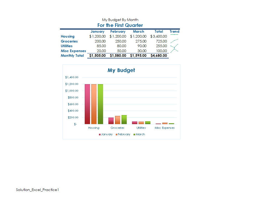
50. Run spelling and grammar check from the Review tab using the Spelling button in the Proofing group, making any spelling corrections as necessary. Compare your file to the image below and make all necessary corrections.
51. Submit as instructed by your instructor.