Excel Practice 6

Here is a video demonstrating the skills in this practice. Please note it does not exactly match the instructions: 

Complete the following Practice Activity and submit your completed project.

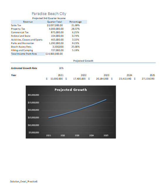
For Excel Practice 6, we will continue to use Excel to manage projected Revenue for Paradise Beach City, where you have just been hired as a Financial Analyst. Key skills in this practice are working with formulas with more than one operator, line graphs and map charts.

1. Start Excel. Click Open, then Browse to where your data files are saved. We will continue working on the same spreadsheet as Excel Practice 5.
2. With the Excel Practice 5 open, Select File, Save As, Browse, and then navigate to your Excel folder on your flash drive or other location where you save your files. Name the workbook as Yourlastname_Yourfirstname_Excel_Practice_6
3. On the Data worksheet, in cell A14 Type Projected Growth. Select the range A14:F14 and merge and center the cells.
4. Apply the cell style Heading 3 to the cell A14.
5. In cell A16 type Estimated Growth Rate and press tab. In cell B16 type .16.
6. Select cell B16 and format it as a percent with zero decimal places.
7. In cell A18 type Year and press tab. In cell B18 type 2021 and press tab. In cell C18 type 2022 and press Enter.
8. With the range B18:C18 selected, use the fill handle to fill the range D18:F18 with the years 2023-2025.
9. In cell B19, enter 15000000 and format it as Accounting Number Format.
10. Apply Bold and Italics formats to cell B16. Use the format painter to apply the same format to cell A18.
11. In cell C19, we will write a formula with multiple operators that calculates the projected growth in expenses with a growth rate of 16% for the years 2022-2015. Parentheses are used to determine the order of operations since there is more than one operator. An absolute reference is used on cell B16. The formula will look like this =B19*(100%+$B$16). Key the formula as shown into cell C19.
12. Since an absolute reference was used on cell B16, we can use the fill handle to fill this formula to cells D19:F19. With Cell C19 selected, use the fill handle to copy the formula to cells D19:F19.
13. Select the columns B:F and autofit the contents.
14. Apply the accounting number format to the range B19:F19 and ensure there are no decimal places. Do not worry if this worksheet is more than one page. We will adjust that at the end.
15. Select the range B18:F19. On the Insert Tab, in the charts group, choose Recommended Charts. Choose the first option which is Line Chart.
16. Move the chart so that the upper left corner is inside cell A21.
17. With the chart selected, change the Chart Title to Projected Growth. Change the font color to Blue Accent1 from the Font group on the Home ribbon using the Font Color button.
18. With the entire chart selected, right-click any of the dollar values and choose Format Axis.
19. In the Format Axis pane, under Bounds, change the Minimum to 5000000. The number will change to scientific notation. Close the Format Axis Pane.
20. With the entire chart selected (not just the axis), on the Chart Tools, Format Tab, in the Shape Styles group, select Shape Fill, and then picture. On the Insert Pictures window, choose From File. Browse to where you store your data files, and select the Beach.jpg picture.
21. With the chart still selected, on the Chart Tools Design tab, choose Quick Styles. Select any Quick Style, or leave the picture as the background.
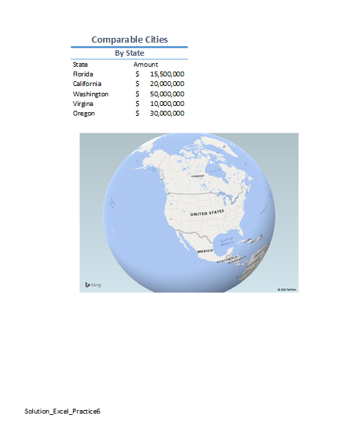
22. Add a new sheet to the workbook and name it Map Chart.
23. In cell A1, type Comparable Cities and press enter.
24. In cell A2 type By State and press Enter.
25. In cell A3 type State and press tab. In cell B3 type Amount and press enter.
26. In cell A4 type Florida and then press Tab and type 15500000 in cell B4 and press Enter.
27. In cell A5 type California and then press Tab and type 20000000 in cell B5 and press Enter.
28. In cell A6 type Washington and then press Tab and type 50000000 in cell B6 and press Enter.
29. In cell A7 type Virginia and then press Tab and type 10000000 in cell B7 and press Enter.
30. In cell A8 type Oregon and then press Tab and type 30000000 in cell B8 and press Enter.
31. Autofit all cell contents.
32. Select the range A1:B1 and merge and center. Apply cell style Heading 1.
33. Select the range A2:B2 and merge and center. Apply cell style Heading 2.
34. Select the range B4:B8 and apply Accounting number format with zero decimal places.
35. On the Insert Tab, in the Tours grouping choose the arrow next to 3D Maps and choose Open 3D Maps.
36. In the 3D Maps window, in the Map group, choose Map Labels.
37. In the Scene group, select Themes, and then choose any Theme.
38. In the Tour group, choose Capture Screen.
39. Return to the Map Chart tab by clicking the File tab and then Close. Next, right click in cell D3 and select paste. This will paste the screenshot into your Map Chart sheet in your workbook.
40. With the Map selected, resize and move the map so that the upper left hand corner is in cell A10 and the lower right hand corner is in cell E26.
41. Group All Sheets.
42. Press Ctrl + F2 to display the Print Preview. Examine all three pages of the workbook, launch the Page Setup Dialog box. On the Page tab, ensure all pages Fit to 1 page.
43. On the Margins tab, center on page horizontally and vertically. You may need to ungroup the sheets in order to do this.
44. On the Header/Footer, ensure Show the file name shows in the left section of the footer in all sheets and click OK to exit the page setup dialog box.
45. In Backstage view select Info, and show the advanced properties. Add the following:
    • Title: Paradise Beach City Analysis with Comparable States
    • Subject: OFTEC 108 (or 100, whichever class you are in) and Section #
    • Author: Your First and Last Name
    • Keywords: Line Charts, Maps and Multiple Operators
46. Run a spelling and grammar check, compare your file to the images below and make all necessary corrections. If necessary, Ungroup the worksheets. Your line chart may vary depending on whether you used the Beach.jpg image as the background or not and you will still have Projected Revenue chart sheet in your workbook (image not shown below of the chart).
47. Submit as instructed by your instructor.