Financial Plan for a Lawn Care Business

Download Data File: PR9 Data

Running your own lawn care business can be an excellent way to make money over the summer while on break from college. It can also be a way to supplement your existing income for the purpose of saving money for retirement or for a college fund. However, managing the costs of the business will be critical in order for it to be a profitable venture. In this exercise you will create a simple financial plan for a lawn care business by using the skills covered in this chapter.

1. Open the file named PR9 Data and then Save As PR9 Lawn Care.
2. Click cell C5 in the Annual Plan worksheet.
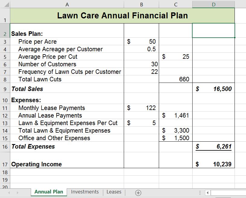
3. Write a formula that calculates the average price per lawn cut.  Do not use the AVERAGE function. The formula should be the Price per Acre multiplied by the Average Acreage per Customer.
4. Click cell C8.
5. Enter a formula that calculates the total number of lawns that will be cut during the year (Number of Customers * Frequency of Lawn Cuts per Customer).
6. Click cell D9.
7. Enter a formula that calculates the total sales for the plan (Average Price per Cut * Total Lawn Cuts).
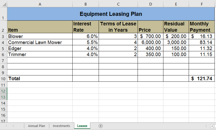
8. Click cell F3 in the Leases worksheet. The PMT function will be used to calculate the monthly lease payment for the first item. For many businesses, leasing (or renting) equipment is a more favorable option than purchasing equipment because it requires far less cash. This enables you to begin a business such as a lawn care business without having to put up a lot of money to buy equipment. The PMT function can be entered using the Insert Function button as seen in Chapter 2, or we can type the PMT function directly into a cell. For this assignment, we will type the function into cell F3 using the following instructions.
9. Type =PMT(   Define the arguments of the function as follows:
   1. Rate: Click cell B3, type a forward slash / for division, type the number 12, and type a comma ,. Since we are calculating monthly payments, the annual interest rate must be converted to a monthly interest rate by dividing by 12.
   2. Nper: Click cell C3, type *12 and then type a comma ,. Similar to the Rate argument, the terms of the lease must be converted to months by multiplying by 12 since we are calculating monthly payments.
   3. Pv: Type a minus sign −, click cell D3, and type a comma ,. Remember that this argument must always be preceded by a minus sign.
   4. Fv: Click cell E3 (Residual Value) and type a comma ,.
   5. Type: Type the number 1, type a closing parenthesis ), and press the ENTER key. We will assume the lease payments will be made at the beginning of each month, which requires that this argument be defined with a value of 1.
10. Copy the PMT function in cell F3 and paste it into the range F4:F6, or use the Autofill handle.
11. Click cell F10 in the Leases worksheet. Enter an Autosum function to calculate the total for the monthly lease payments. Make sure that blank rows (7 through 9) were included in the range for the SUM function. If other items are added to the worksheet, they will be included in the output of the SUM function.
12. Highlight the range A2:F6 on the Leases worksheet. The data in this range will be sorted, first by Interest Rate and then by Price. Click the Sort button in the Data tab of the Ribbon. In the Sort dialog box, select the Interest Rate option in the “Sort by” drop-down box. Select Largest to Smallest for the sort order. Then, click the Add Level button on the Sort dialog box. Select the Price option in the “Then by” drop-down box. Select Largest to Smallest for the sort order. Click the OK button in the Sort dialog box.
13. Click cell B11 on the Annual Plan worksheet. The monthly lease payments that are calculated in the Lease worksheet will be displayed in this cell.
14. Type an equal sign =. Click the Leases worksheet, click cell F10, and press the ENTER key.
15. Click cell C12 on the Annual Plan worksheet. Create a formula that calculates the annual lease payments. This should be the Monthly Lease Payments * 12.
16. Click cell C14 on the Annual Plan worksheet. Create a formula that calculates the Total Lawn & Equipment Expenses (Lawn & Equipment Expenses per Cut * Total Lawn Cuts).
17. Click cell D16 on the Annual Plan worksheet. Enter a SUM function that adds the Expenses for the business in column C. Make sure to add the Expenses only (not the Sales Plan information).
18. Click cell D17 on the Annual Plan worksheet. Enter a formula that calculates the annual profit (Operating Income) for the business. This should be the Total Sales – Total Expenses.
19. Format all cells that contain money amounts in the Annual Plan worksheet for Accounting Number Format ($) with no decimals.
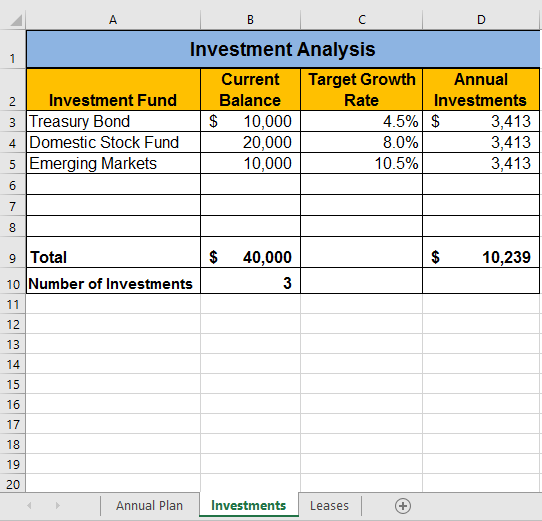
20. Click cell B10 on the Investments worksheet. Enter a COUNT function that counts the number of investments that currently have a balance in column B. Make sure that the additional blank rows in rows 6 through 8 are included in the range for this function. The function output will automatically change if any new investments are added to the worksheet. It is important to note, however, that the Total in cell B9 should not be included in the Count range.
21. Click cell D3 on the Investments worksheet.
22. Type an equal sign =. Click the Annual Plan worksheet. Click cell D17 and type a forward slash / for division. Click the Investments worksheet. Click cell B10 and press the ENTER key. This formula divides the profit calculated on the Annual Plan worksheet by the number of investments in the Investments worksheet. We will assume that the profits from this business will be invested evenly among the funds listed in Column A of the Investments worksheet.
23. Before copying and pasting the formula created in cell D3, absolute references must be added to the cell locations in the formula. Edit the formula in cell D3 on the Investments worksheet so that cells D17 and B10 are absolute. The formula in cell D3 should be: =’Annual Plan’!$D$17/Investments!$B$10. When you copy the formula in cell D3 down, the cell references will not change, because they are absolute. The formula will continue to divide the Operating Income in cell D17 of the Annual Plan by the Number of Investments in cell B10 of the Investments sheet.
24. Copy cell D3 and paste it into cells D4 and D5 or use the Auto Fill handle to copy down.
25. Click cell B9 on the Investments worksheet. Enter a SUM function that adds the current balance for all investments in column B. Make sure that blank rows (rows 6 through 8) are added to the range for the function so additional investments will automatically be included in the Autosum function output.
26. Copy the SUM function in cell B9 and paste it into cell D9.
27. Format the Investments and Leases sheets appropriately for Accounting Format. This should include $ signs on the top row and total row for money amounts, and comma style in the middle rows. In the Investments sheet, apply Comma Style with 0 decimals to the ranges B4:B5 and D4:D5. In the Leases worksheet, apply Accounting Number Format ($) with two decimals to the range D3:F3 and F10. Apply comma format with two decimals to the range D4:F9. Double check that your formatting matches Figures 2.47a through 2.47c.
28. Save the PR2 Lawn Care workbook.

Attribution

Adapted by Mary Schatz from How to Use Microsoft Excel: The Careers in Practice Series, adapted by The Saylor Foundation without attribution as requested by the work’s original creator or licensee, and licensed under CC BY-NC-SA 3.0.