
13 3.1 More on Formulas and Functions
Learning Objectives
- Review the use of the =MAX function.
- Examine the Quick Analysis Tool to create standard calculations, formatting, and charts very quickly.
- Create Percentage calculation.
– Use the Smart Lookup tool to acquire additional information about percentage calculations.
– Review the use of Absolute cell reference in a division formula.
Another use for =MAX
Before we move on to the more interesting calculations we will be discussing in this chapter, we need to determine how many points it is possible for each student to earn for each of the assignments. This information will go into Row 25. The =MAX function is our tool of choice.
Download Data File: CH3 Data
- Open the data file CH3 Data and save the file to your computer as CH3 Gradebook and Parks.
- Make B25 your active cell.
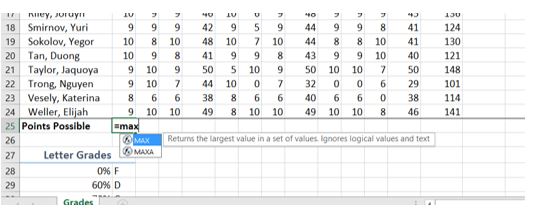
- Start typing =MAX (See Figure 3.2) Note the explanation you see on the offered list of functions. You can either keep typing ( or double click MAX from the list.

Figure 3.2 Entering a function - Select the range of numbers above row 25. Your calculation will be: =MAX(B5:B24).
- Press Enter after selecting the range.
- Now, use the Fill Handle to copy the calculation from Column B through Column N.
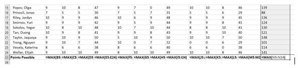
Note that as you copy the calculation from one column to the next, the cell references change. The calculation in column B reads: =MAX(B5:B24). The one in column N reads: =MAX(N5:N24). These cell references are relative references.
By default, the calculations that Excel copies change their cell references relative to the row or column you copy them to. That makes sense. You wouldn’t want column N to display an answer that uses the values in column L.
Want to see all the calculations you have just created? Press Ctrl ~ (See Figure 3.3.) Ctrl ~ displays your calculations (formulas). Pressing Ctrl ~ a second time will display your calculations in the default view – as values.
Quick Analysis Tool
The Quick Analysis Tool allows you to create standard calculations, formatting, and charts very quickly. In this exercise we will use it to insert the Total Points for each student in Column O.
![]() Mac Users: the Quick Analysis Tool is not available with Excel for Mac. We have alternate steps for Mac Users below. Skip down below Figure 3.5 to continue.)
Mac Users: the Quick Analysis Tool is not available with Excel for Mac. We have alternate steps for Mac Users below. Skip down below Figure 3.5 to continue.)
Be sure to press Ctrl ~ to return your spreadsheet to the normal view (the formula results should display, not the formulas themselves).
- Select the range of cells B5:N25
- In the lower right corner of your selection, you will see the Quick Analysis tool (see Figure 3.4).
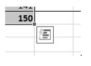
Figure 3.4 Quick Analysis Tool - When you click on it, you will see that there are a number of different options. This time we will be using the Totals option. In future exercises, we will use other options.
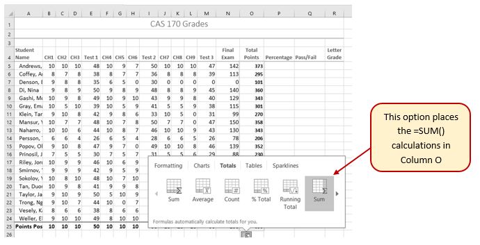
- Select Totals, and then the SUM option that highlights the right column (see Figure 3.5). Selecting that SUM option places =SUM() calculations in column O.

![]() Alternate steps for Mac Users:
Alternate steps for Mac Users:
- Select the range B5:O25 then click the AutoSum button on the Ribbon (Home tab or Formulas tab)
- Select the range O5:O25 and click the Bold button.
Percentage calculation
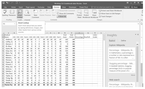
Column P requires a Percentage calculation. Before we launch into creating a calculation for this, it might be handy to know precisely what it is we are looking for. If you are connected to the internet and are using Excel 365, you can use the Smart Lookup tool to get some more information about calculating percentages.
In general, the Smart Lookup tool allows you to get more information and definitions about unfamiliar terms or features. This tool is available in all of the Microsoft Office applications.
- Select cell P4.
- Find the Smart Lookup tool on the Review tab (see Figure 3.6) and click it. You can also “Right-click” the specific cell and choose Smart Lookup.
 Mac Users: The Smart Lookup tool is only on the Review tab in the latest versions of Excel for Mac. If you can’t find the Smart Lookup tool on the Review tab, you will find it by clicking on the “Tools” menu bar option.
Note for all users: there is a keyboard shortcut for using the Smart Lookup tool. You can hold down the Control key and click in the specific cell (in this case, P4) - If this is the first time you have used the Smart Lookup tool, you may need to respond to a statement about your privacy. Press the Got it button. We think the Wikipedia article does a pretty good job explaining the calculation, don’t you?
- Close the Smart Lookup pane after reading through the definitions.
Now that we know what is needed for the Percentage calculation, we can have Excel do the calculation for us. We need to divide the Total Points for each student by the Total Points of all the Points Possible. Notice that there is a different number on each row – for each student. But, there is only one Total Points Possible – the value that is in cell O25.
- Make sure that P5 is your active cell.
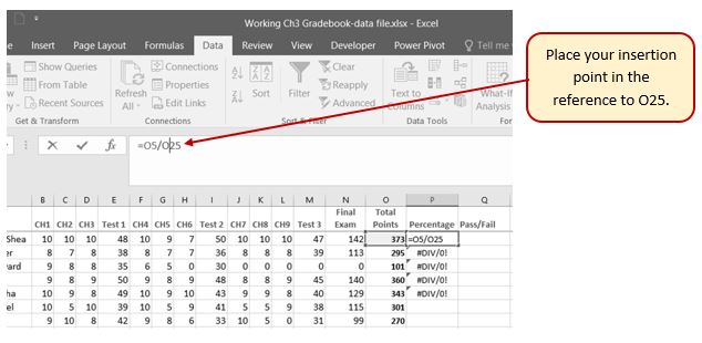
- Press = then select cell O5. Press /, then cell O25. Your calculation should look like this: =O5/O25. The result of the formula should be 0.95641026. (So far, so good. DeShea Andrews is doing well in this class – with a percentage grade of almost 96%. Definitely an “A”!)
- Next use the Fill handle to copy the calculation down through row 24 to calculate the other students’ grades. You should get the error message #DIV/0!. This error message reminds us that you can’t divide a number by 0 (zero). And that is just what is happening. If you look at the calculation in P9, the calculation reads: =O9/O29. The first cell reference is correct – it points to Moesha Gashi’s total points for the class. But the second reference is wrong. It points to an empty cell – O29.
Before copying the calculation, we have to make the second reference (O25) an absolute cell reference. That way, when we copy the formula down, the cell reference for O25 will be locked and will not change.
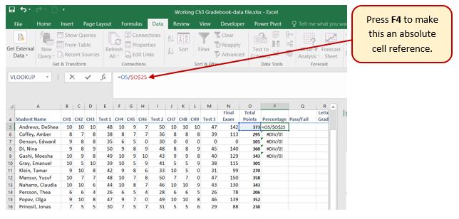
- Make P5 your active cell. In the Formula Bar click on O25 (see Figure 3.7).
- Press F4 (on the function keys at the top of your keyboard). That will make the O25 reference absolute. It will not change when you copy the calculation (see Figure 3.8). (If you are working on a laptop and do not have an F4 function key, you can type in a $ before the O and another one before the 25.)
- The calculation now looks like this: =O5/$O$25.
- Use the Fill Handle to copy the formula down through P24 again. Now, when you copy the formula, you will get correct values for all of the students.
Those long decimals are a bit nonstandard. Let’s change them to % by applying cell formatting.
- Select the range P5:P24.
- On the Home tab, in the Number Group, select the % (Percent Style) button.
Skill Refresher
Absolute References
- Click in front of the column letter of a cell reference in a formula or function that you do not want altered when the formula or function is pasted into a new cell location.
- Press the F4 key or type a dollar sign ($) in front of the column letter and row number of the cell reference.
Keyboard Shortcuts
Smart Lookup Tool
- Hold down the CTRL key and click the specific cell that you are working with. Then choose “Smart Lookup“
- Mac Users: Same as above
Key Takeaways
- Functions can be created using cell ranges or selected cell locations separated by commas. Make sure you use a cell range (two cell locations separated by a colon) when applying a statistical function to a contiguous range of cells.
- To prevent Excel from changing the cell references in a formula or function when they are pasted to a new cell location, you must use an absolute reference. You can do this by placing a dollar sign ($) in front of the column letter and row number of a cell reference or by using the F4 function key.
- The #DIV/0 error appears if you create a formula that attempts to divide a constant or the value in a cell reference by zero.
More functions:
Create the Sample Worksheet
This section uses a sample worksheet to illustrate Excel built-in functions. Consider the example of referencing a name from column A and returning the age of that person from column C. To create this worksheet, enter the following data into a blank Excel worksheet.
You will type the value that you want to find into cell E2. You can type the formula in any blank cell in the same worksheet.
| A | B | C | D | E | ||
| 1 | Name | Dept | Age | Find Value | ||
| 2 | Henry | 501 | 28 | Mary | ||
| 3 |
Stan |
201 | 19 | |||
| 4 | Mary | 101 | 22 | |||
| 5 | Larry | 301 |
29 |
| Term | Definition | Example |
| Table Array | The whole lookup table | A2:C5 |
| Lookup_Value | The value to be found in the first column of Table_Array. | E2 |
| Lookup_Array -or- Lookup_Vector |
The range of cells that contains possible lookup values. | A2:A5 |
| Col_Index_Num | The column number in Table_Array the matching value should be returned for. | 3 (third column in Table_Array) |
| Result_Array -or- Result_Vector |
A range that contains only one row or column. It must be the same size as Lookup_Array or Lookup_Vector. | C2:C5 |
| Range_Lookup | A logical value (TRUE or FALSE). If TRUE or omitted, an approximate match is returned. If FALSE, it will look for an exact match. | FALSE |
| Top_cell | This is the reference from which you want to base the offset. Top_Cell must refer to a cell or range of adjacent cells. Otherwise, OFFSET returns the #VALUE! error value. | |
| Offset_Col
CONCAT |
This is the number of columns, to the left or right, that you want the upper-left cell of the result to refer to. For example, “5” as the Offset_Col argument specifies that the upper-left cell in the reference is five columns to the right of reference. Offset_Col can be positive (which means to the right of the starting reference) or negative (which means to the left of the starting reference).
This is used for text that needs to be merged into one cell. You can type data into cells, then by using the CONCAT function and the range or cells you want to use, the data will be merged into the cell reference. For example, if you have the words “Red” in cell C2 and “Cat” in cell C3, by using CONCAT in cell C4, you can have the words Red Cat appear in that cell. |
Functions
LOOKUP()
The LOOKUP function finds a value in a single row or column and matches it with a value in the same position in a different row or column.
The following is an example of LOOKUP formula syntax:
=LOOKUP(Lookup_Value,Lookup_Vector,Result_Vector)
The following formula finds Mary’s age in the sample worksheet:
=LOOKUP(E2,A2:A5,C2:C5)
The formula uses the value “Mary” in cell E2 and finds “Mary” in the lookup vector (column A). The formula then matches the value in the same row in the result vector (column C). Because “Mary” is in row 4, LOOKUP returns the value from row 4 in column C (22).
NOTE: The LOOKUP function requires that the table be sorted.
For more information about the LOOKUP function, click the following article number to view the article in the Microsoft Knowledge Base:
How to use the LOOKUP function in Excel
VLOOKUP()
The following formula finds Mary’s age in the sample worksheet:
=VLOOKUP(E2,A2:C5,3,FALSE)
The formula uses the value “Mary” in cell E2 and finds “Mary” in the left-most column (column A). The formula then matches the value in the same row in Column_Index. This example uses “3” as the Column_Index (column C). Because “Mary” is in row 4, VLOOKUP returns the value from row 4 in column C (22).
For more information about the VLOOKUP function, click the following article number to view the article in the Microsoft Knowledge Base:
How to Use VLOOKUP or HLOOKUP to find an exact match
INDEX() and MATCH()
The following formula finds Mary’s age in the sample worksheet:
=INDEX(A2:C5,MATCH(E2,A2:A5,0),3)
The formula uses the value “Mary” in cell E2 and finds “Mary” in column A. It then matches the value in the same row in column C. Because “Mary” is in row 4, the formula returns the value from row 4 in column C (22).
NOTE: If none of the cells in Lookup_Array match Lookup_Value (“Mary”), this formula will return #N/A.
For more information about the INDEX function, click the following article number to view the article in the Microsoft Knowledge Base:
How to use the INDEX function to find data in a table
OFFSET() and MATCH()
This formula finds Mary’s age in the sample worksheet:
=OFFSET(A1,MATCH(E2,A2:A5,0),2)
The formula uses the value “Mary” in cell E2 and finds “Mary” in column A. The formula then matches the value in the same row but two columns to the right (column C). Because “Mary” is in column A, the formula returns the value in row 4 in column C (22).
For more information about the OFFSET function, click the following article number to view the article in the Microsoft Knowledge Base:
Using the some of the functions exercise
To complete this assignment, you will be required to use this data file: SC_EX_3.1b
- Start Excel and open the workbook in the datafile3.1b.xlsx. This workbook contains loan information for which you will create a loan payment calculator.
- Select the range b4:c9, Use the “Create from Selection button (Formulas tab | Defined Names group) to create names for the cells in range C4:C9 using the row titles in the range B4:B9.
- Enter the formulas shown in the table below
| Cell | Formula |
| C8
C9 F4 G4 H4 |
=Price-Down_Payment =-PMT(Interest_Rate/12, 12*Years, Loan_Amount) =Monthly_Payment =12*Monthly_Payment*Years=Down_Payment =G4-Price
|
- Use the Data Table button in the What-If Analysis gallery (Data tab | Forecast group) to define the range E4:H19 as a one-input data table. Use the Interest Rate in the Laon Payment Calculator as the column input cell.
- Use the Page Setup dialog box to select the Fit to and “Black and White” options. Select the range B2:C9 and then use the “Set Print Area” command to set a print area. Use the Print button on the Print Screen in Backstage view to print the worksheet. Use the “Clear Print Area” command to clear the print area.
- Name the following ranges: B2:C9-Calculator; E2:H19-Raqte_Scheudle: and B2:H19-All_Section. Print each range by selecting the name in the Name box and using the print Selection optoin on the Print screen in backstage view.
- Unlock the range C3:C7. Protect the worksheet so that the user can select only unlocked cells (challenge).
- Press CTRL+` and then print the formulas verson in landscape orientation. Press CTRL+` again to return to the values version.
- Hide and then unhide the Laon Payment Calculator workshee4t. Hide and then unhide the workbook. Delete the extra worksheet you made so you can hide the loan payment Calculator worksheet. Unprotect the worksheet and then hide columns E through H. Select columns D and I and reveal the hidden columns. Hide rows 11 through 19. Print the worksheet (Use print screen or create a print screen PDF from the Print options). Select rows 10 and 20 and unhide rows 11 through 19. Protect the worksheet.
- Copy the data from the car worksheet to a new worksheet. Determine the monthly payment and print the worksheet for each data set and set each to a new worksheet: (a) Item=Motorhome; Down payment = $75,000.00; Price = $225,000; Years = 7; Interest rate = 8.00; (b) Item=Debt Consolidation Loan; Down Payment – $0.0; Price = $40,000.00; Years =5; Interest rate = 11.35. Label each sheet tab with an appropriate label for each calculations set and add your initials to each worksheet tab.
- Save the workbook with the file name, SC_EX_4_Loan+ your initials and upload to the assignment specified by your instructor.
Attribution
3.1 More on Formulas and Functions by Noreen Brown, Mary Schatz, and Art Schneider, Portland Community College, is licensed under CC BY 4.0
Support.microsoft.com and Jennifer Evans, South Puget Sound Community College, is licensed under CC by 4.0
