LO 2.3 Estimate a Variable and Fixed Cost Equation and Predict Future Costs
Sometimes, a business will need to use cost estimation techniques, particularly in the case of mixed costs, so that they can separate the fixed and variable components, since only the variable components change in the short run. Estimation is also useful for using current data to predict the effects of future changes in production on total costs. Three estimation techniques that can be used include the scatter graph, the high-low method, and regression analysis. Here we will demonstrate the scatter graph and the high-low methods (you will learn the regression analysis technique in advanced managerial accounting courses.
Functions of Cost Equations
The cost equation is a linear equation that takes into consideration total fixed costs, the fixed component of mixed costs, and variable cost per unit. Cost equations can use past data to determine patterns of past costs that can then project future costs, or they can use estimated or expected future data to estimate future costs. Recall the mixed cost equation:

where Y is the total mixed cost, a is the fixed cost, b is the variable cost per unit, and x is the level of activity.
Let’s take a more in-depth look at the cost equation by examining the costs incurred by Eagle Electronics in the manufacture of home security systems, as shown in (Figure).
| Cost Information for Eagle Electronics | ||
|---|---|---|
| Cost Incurred | Fixed or Variable | Cost |
| Lease on manufacturing equipment | Fixed | $50,000 per year |
| Supervisor salary | Fixed | $75,000 per year |
| Direct materials | Variable | $50 per unit |
| Direct labor | Variable | $20 per unit |
By applying the cost equation, Eagle Electronics can predict its costs at any level of activity (x) as follows:
- Determine total fixed costs: $50,000 + $75,000 = $125,000
- Determine variable costs per unit: $50 + $20 = $70
- Complete the cost equation: Y = $125,000 + $70x
Using this equation, Eagle Electronics can now predict its total costs (Y) for any given level of activity (x), as in (Figure):

When using this approach, Eagle Electronics must be certain that it is only predicting costs for its relevant range. For example, if they must hire a second supervisor in order to produce 12,000 units, they must go back and adjust the total fixed costs used in the equation. Likewise, if variable costs per unit change, these must also be adjusted.
This same approach can be used to predict costs for service and merchandising firms, as shown by examining the costs incurred by J&L Accounting to prepare a corporate income tax return, shown in (Figure).
| Cost Information for J&L Accounting | ||
|---|---|---|
| Cost Incurred | Fixed or Variable | Cost |
| Building rent | Fixed | $1,000 per month |
| Direct labor (for CPAs) | Variable | $250 per tax return |
| Secretarial staff | Fixed | $2,000 per month |
| Accounting clerks | Variable | $100 per return |
J&L wants to predict their total costs if they complete 25 corporate tax returns in the month of February.
- Determine total fixed costs: $1,000 + $2,000 = $3,000
- Determine variable costs per tax return: $250 + $100 = $350
- Complete the cost equation: Y = $3,000 + $350x
Using this equation, J&L can now predict its total costs (Y) for the month of February when they anticipate preparing 25 corporate tax returns:
J&L can now use this predicted total cost figure of $11,750 to make decisions regarding how much to charge clients or how much cash they need to cover expenses. Again, J&L must be careful to try not to predict costs outside of the relevant range without adjusting the corresponding total cost components.
J&L can make predictions for their costs because they have the data they need, but what happens when a business wants to estimate total costs but has not collected data regarding per-unit costs? This is the case for the managers at the Beach Inn, a small hotel on the coast of South Carolina. They know what their costs were for June, but now they want to predict their costs for July. They have gathered the information in (Figure).
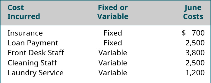
In June, they had an occupancy of 75 nights. For the Beach Inn, occupancy (rooms rented) is the cost driver. Since they know what is driving their costs, they can determine their per-unit variable costs in order to forecast future costs:
Now, the Beach Inn can apply the cost equation in order to forecast total costs for any number of nights, within the relevant range.
- Determine total fixed costs: $700 + $2,500 = $3,200
- Determine variable costs per night of occupancy: $50.67 + $33.33 + $16.00 = $100
- Complete the cost equation: Y = $3,200 + $100x
Using this equation, the Beach Inn can now predict its total costs (Y) for the month of July, when they anticipate an occupancy of 93 nights.
In all three examples, managers used cost data they have collected to forecast future costs at various activity levels.
YOUR TURN
Waymaker Furniture has collected cost information from its production process and now wants to predict costs for various levels of activity. They plan to use the cost equation to formulate these predictions. Information gathered from March is presented in (Figure).
| March Cost Information for Waymaker Furniture | ||
|---|---|---|
| Cost Incurred | Fixed or Variable | March Cost |
| Plant supervisor salary | Fixed | $12,000 per month |
| Lumber (direct materials) | Variable | $75,000 total |
| Production worker wages | Variable | $11.00 per hour |
| Machine maintenance | Variable | $5.00 per unit produced |
| Lease on factory | Fixed$ | 15,000 per month |
In March, Waymaker produced 1,000 units and used 2,000 hours of production labor.
Using this information and the cost equation, predict Waymaker’s total costs for the levels of production in (Figure).
| Waymaker’s Levels of Production | |
|---|---|
| Month | Activity Level |
| April | 1,500 units |
| May | 2,000 units |
| June | 2,500 units |
Solution
Total Fixed Cost = $12,000 + $15,000 = $27,000. Direct Materials per Unit = $75,000 / 1,000 Units = $75 per unit. Direct Labor per Hour = $11.00. Machine Maintenance = $5.00 per unit. Total Variable Cost per Unit = $75 + $11 + $5 = $91 per unit.

Demonstration of the Scatter Graph Method to Calculate Future Costs at Varying Activity Levels
One of the assumptions that managers must make in order to use the cost equation is that the relationship between activity and costs is linear. In other words, costs rise in direct proportion to activity. A diagnostic tool that is used to verify this assumption is a scatter graph.
A scatter graph shows plots of points that represent actual costs incurred for various levels of activity. Once the scatter graph is constructed, we draw a line (often referred to as a trend line) that appears to best fit the pattern of dots. Because the trend line is somewhat subjective, the scatter graph is often used as a preliminary tool to explore the possibility that the relationship between cost and activity is generally a linear relationship. When interpreting a scatter graph, it is important to remember that different people would likely draw different lines, which would lead to different estimations of fixed and variable costs. No one person’s line and cost estimates would necessarily be right or wrong compared to another; they would just be different. After using a scatter graph to determine whether cost and activity have a linear relationship, managers often move on to more precise processes for cost estimation, such as the high-low method or least-squares regression analysis.
To demonstrate how a company would use a scatter graph, let’s turn to the data for Regent Airlines, which operates a fleet of regional jets serving the northeast United States. The Federal Aviation Administration establishes guidelines for routine aircraft maintenance based upon the number of flight hours. As a result, Regent finds that its maintenance costs vary from month to month with the number of flight hours, as depicted in (Figure).
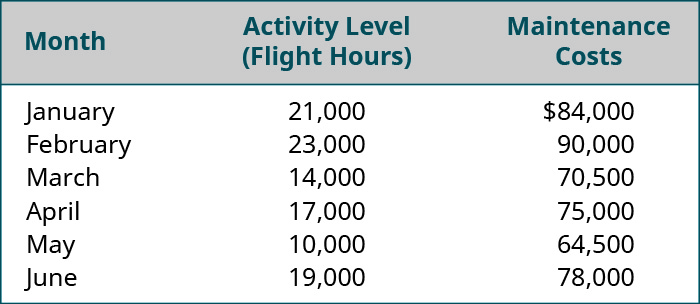
When creating the scatter graph, each point will represent a pair of activity and cost values. Maintenance costs are plotted on the vertical axis (Y), while flight hours are plotted on the horizontal axis (X). For instance, one point will represent 21,000 hours and $84,000 in costs. The next point on the graph will represent 23,000 hours and $90,000 in costs, and so forth, until all of the pairs of data have been plotted. Finally, a trend line is added to the chart in order to assist managers in seeing if there is a positive, negative, or zero relationship between the activity level and cost. (Figure) shows a scatter graph for Regent Airlines.
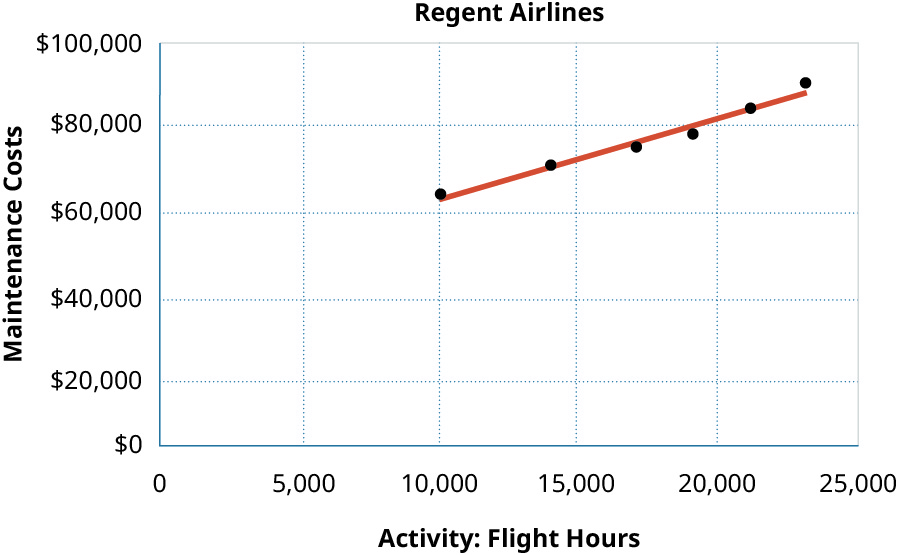
In scatter graphs, cost is considered the dependent variable because cost depends upon the level of activity. The activity is considered the independent variable since it is the cause of the variation in costs. Regent’s scatter graph shows a positive relationship between flight hours and maintenance costs because, as flight hours increase, maintenance costs also increase. This is referred to as a positive linear relationship or a linear cost behavior.
Will all cost and activity relationships be linear? Only when there is a relationship between the activity and that particular cost. What if, instead, the cost of snow removal for the runways is plotted against flight hours? Suppose the snow removal costs are as listed in (Figure).
| Snow Removal Costs | ||
|---|---|---|
| Month | Activity Level: Flight Hours | Snow Removal Costs |
| January | 21,000 | $40,000 |
| February | 23,000 | 50,000 |
| March | 14,000 | 8,000 |
| April | 17,000 | 0 |
| May | 10,000 | 0 |
| June | 19,000 | 0 |
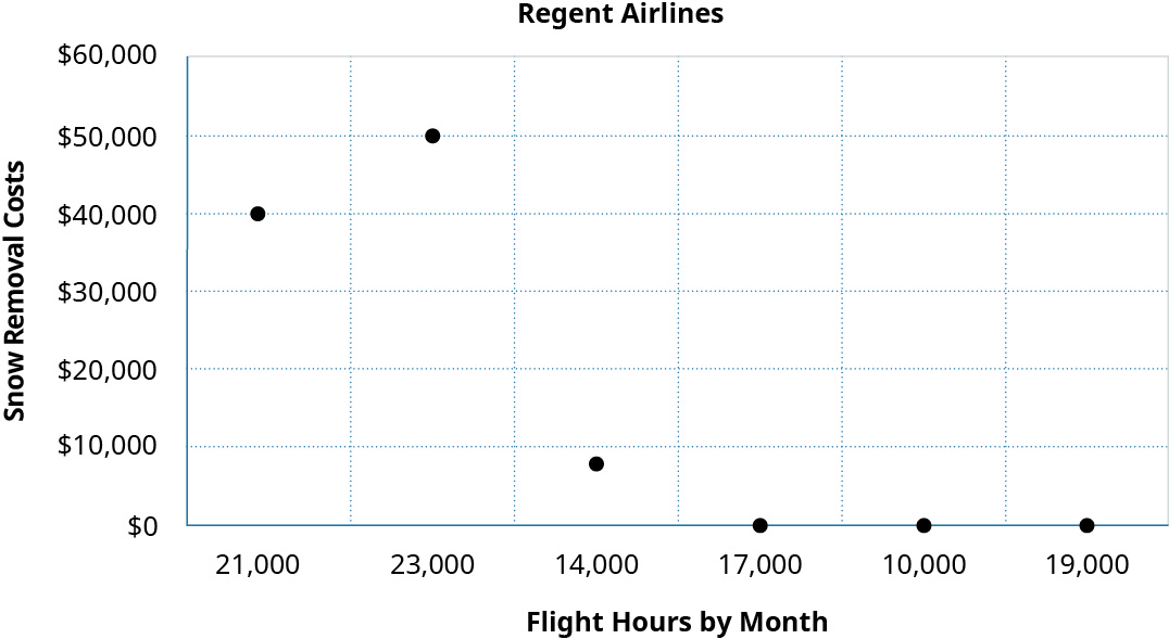
As you can see from the scatter graph, there is really not a linear relationship between how many flight hours are flown and the costs of snow removal. This makes sense as snow removal costs are linked to the amount of snow and the number of flights taking off and landing but not to how many hours the planes fly.
Using a scatter graph to determine if this linear relationship exists is an essential first step in cost behavior analysis. If the scatter graph reveals a linear cost behavior, then managers can proceed with a more sophisticated analyses to separate mixed costs into their fixed and variable components. However, if this linear relationship is not present, then other methods of analysis are not appropriate. Let’s examine the cost data from Regent Airline using the high-low method.
Demonstration of the High-Low Method to Calculate Future Costs at Varying Activity Levels
As you’ve learned, the purpose of identifying costs is to control them, and managers regularly use past costs to predict future costs. Since we know that variable costs change with the level of activity, we can conclude that there is usually a positive relationship between cost and activity: As one rises, so does the other. Ideally, this can be confirmed on a scatter graph. One of the simplest ways to analyze costs is to use the high-low method, a technique for separating the fixed and variable cost components of mixed costs. Using the highest and lowest levels of activity and their associated costs, we are able to estimate the variable cost components of mixed costs.
Once we have established that there is linear cost behavior, we can equate variable costs with the slope of the line, expressed as the rise of the line over the run. The steeper the slope of the line, the faster costs rise in response to a change in activity. Recall from the scatter graph that costs are the dependent Y variable and activity is the independent X variable. By examining the change in Y relative to the change in X, we can predict cost:

where Y2 is the total cost at the highest level of activity; Y1 is the total cost at the lowest level of activity; X2 is the number of units, labor hours, etc., at the highest level of activity; and X1 is the number of units, labor hours, etc., at the lowest level of activity.
Using the maintenance cost data from Regent Airlines shown in (Figure), we will examine how this method works in practice.
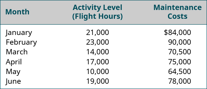
The first step in analyzing mixed costs with the high-low method is to identify the periods with the highest and lowest levels of activity. In this case, it would be February and May, as shown in (Figure). We always choose the highest and lowest activity and the costs that correspond with those levels of activity, even if they are not the highest and lowest costs.

We are now able to estimate the variable costs by dividing the difference between the costs of the high and the low periods by the change in activity using this formula:

For Regent Airlines, this is:
Having determined that the variable cost per flight-hour is $1.96, we can now determine the amount of fixed costs. We can determine these fixed costs by taking the total costs at either the high or the low level of activity and subtracting this variable component. You will recall that total cost = fixed costs + variable costs, so the fixed cost component for Regent Airlines can be isolated as shown:
Notice that if we had chosen the other data point, the low cost and activity, we would still get the same fixed cost of $44,920 = [$64,500 minus (10,000 times $1.96)].
Now that we have isolated both the fixed and the variable components, we can express Regent Airlines’ cost of maintenance using the total cost equation:
where Y is total cost and x is flight hours.
Because we confirmed that the relationship between cost and activity at Regent exhibits linear cost behavior on the scatter graph, this equation allows managers at Regent Airlines to conclude that for every one unit increase in activity, there will be a corresponding rise in variable cost of $1.96. When put into practice, the managers at Regent Airlines can now predict their total costs at any level of activity, as shown in (Figure).

Although managers frequently use this method, it is not the most accurate approach to predicting future costs because it is based on only two pieces of cost data: the highest and the lowest levels of activity. Actual costs can vary significantly from these estimates, especially when the high or low activity levels are not representative of the usual level of activity within the business. For a more accurate model, the least-squares regression method would be used to separate mixed costs into their fixed and variable components. The least-squares regression method is a statistical technique that may be used to estimate the total cost at the given level of activity based on past cost data. Least-squares regression minimizes the errors of trying to fit a line between the data points and thus fits the line more closely to all the data points.
Understanding the various labels used for costs is the first step toward using costs to evaluate business decisions. You will learn more about these various labels and how they are applied in decision-making processes as you continue your study of managerial accounting in this course.
KEY TAKEAWAYS
Key Concepts and Summary
- In order to make business decisions, managers can utilize past cost data to predict future costs employing three methods: scatter graphs, the high-low method, and least-squares regression analysis.
- Scatter graphs are used as a diagnostic tool to determine if the relationship between activity and cost is a linear relationship.
- Both the high-low method and the least-squares regression method separate mixed costs into their fixed and variable components to allow managers to predict future costs from historical costs.
Glossary
- high-low method
- technique for separating the fixed and variable cost components of mixed costs
- scatter graph
- plot of pairs of numerical data that represents actual costs incurred for various levels of activity, with one variable on each axis, used to determine whether there is a relationship between them
Adapted from Principles of Accounting, Volume 2: Managerial Accounting (c) 2019 by Open Stax. The textbook content was produced by Open Stax and is licensed under a Creative Commons BY-NC-SA 4.0 license. Download for free at https://openstax.org/details/books/principles-managerial-accounting
